Solution Walkthrough: Visualizing Daily Cloud Spend on GCP using GKE, Dataflow, BigQuery and Grafana


For any successful cloud adoption, gaining comprehensive visibility into ongoing cloud spend is essential - no one wants to receive a bill higher than expected when trying to plan a budget.
In the case of Google Cloud Platform, there are different charging models for different resources. For example, GCE cost depends on machine type (based on CPU, memory, network and disks), Google Kubernetes Engine (GKE) and Google Cloud Dataproc charges are based on all running nodes on Google Compute Engine (GCE), while some other service costs have more complex formulas. It becomes increasingly difficult to predict cloud spends, especially when you use a lot of different resources. It is important to be aware of the spending and be able to respond in time if it becomes too expensive. If you can proactively monitor billing reports every day, the probability of receiving a surprising bill at the end of the month is drastically reduced.
In a recent project, we wanted to implement an extended billing report functionality to efficiently track spending. While GCP allows exporting billing data into BigQuery for further comprehensive analysis, manually querying BigQuery tables is unlikely sufficient enough; ideally, an operator is able to visualise data and to filter and aggregate by additional parameters. The most common filters are resource type, time period, team and department, and comparison with previous periods.
The first solution we tried was based on Google’s suggestions to use Google Data Studio. While the implementation was very straightforward because of the sample reports and dashboards already available, and only data source configurations were required, the solution was not flexible enough. At creating a chart in Google Data Studio, the user needs to choose all parameters manually instead of providing a formula. To make the billing report more user-friendly we decided to look for another way.
Based on our previous experience we thought that Grafana would be a good option to visualise billing data if we could find a way to connect it to BigQuery (BQ). We tried an open-source BQ plugin for Grafana, but it contained a lot of bugs and was not stable enough. Additionally, there was another issue - BQ jobs take too much time to return data.
Eventually, we decided to load data to PostgreSQL in CloudSQL (because CloudSQL is the easiest way to have a relational database instance) and use Grafana for visualisation. Grafana has an official PostgreSQL plugin, we tested it and realized that it was the best fit to our requirements.
Solution Overview
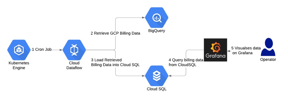
The diagram below is an overview to the workflow we implemented. We deployed a cronjob to the Kubernetes cluster that triggered a Cloud Dataflow job every 4 hours. The dataflow job initiated data loading from BQ to PostgreSQL. It checked max(export_time) in PostgreSQL and loaded data from BQ incrementally, i.e.only importing the data since the last BQ export. The end-users could monitor Grafana dashboards connected to the PostgreSQL instance for the latest billing data.
Setting up the Database
Export Billing Data to BigQuery
First, we set up billing data export to BigQuery, as described here.
Create a PostgresQL Database
The easiest way to create a PostgreSQL instance is by using Cloud SQL.
After the instance was up and running, we created a number of database objects, including a table that mimicked the BQ table structure and a materialized view with indexes that we would use for connecting to PostgreSQL from Grafana.
CREATE DATABASE billing;
USE billing;

CREATE TABLE public.billing_export_2 (
    id serial NOT NULL,
    sku_id varchar NULL,
    labels varchar NULL,
    export_time varchar NULL,
    currency varchar NULL,
    sku_description varchar NULL,
    location_zone varchar NULL,
    currency_conversion_rate float8 NULL,
    project_labels varchar NULL,
    location_country varchar NULL,
    usage_start_time varchar NULL,
    billing_account_id varchar NULL,
    location_region varchar NULL,
    usage_pricing_unit varchar NULL,
    usage_amount_in_pricing_units float8 NULL,
    cost_type varchar NULL,
    project_id varchar NULL,
    system_labels varchar NULL,
    project_description varchar NULL,
    location_location varchar NULL,
    project_ancestry_numbers varchar NULL,
    credits varchar NULL,
    service_description varchar NULL,
    usage_amount float8 NULL,
    invoice_month varchar NULL,
    usage_unit varchar NULL,
    usage_end_time varchar NULL,
    "cost" float8 NULL,
    service_id varchar NULL,
    CONSTRAINT billing_export_2_pkey PRIMARY KEY (id)
);
It is a good practice to add a minimal set of labels to all resources. Every label from this set is represented as a separate column in the view. We also created indexes on these columns to make the Grafana queries faster.
CREATE MATERIALIZED VIEW vw_billing_export AS
    SELECT
        id,
        sku_id,
        labels,
        export_time::timestamp,
        currency,
        sku_description,
        location_zone,
        currency_conversion_rate,
        project_labels,
        location_country,
        usage_start_time::timestamp,
        billing_account_id,
        location_region,
        usage_pricing_unit,
        usage_amount_in_pricing_units,
        cost_type, project_id,
        system_labels,
        project_description,
        location_location,
        project_ancestry_numbers,
        credits,
        service_description,
        usage_amount,
        invoice_month,
        usage_unit,
        usage_end_time::timestamp,
        "cost",
        service_id,
        l_label1 ->> 'value' as label1,
        l_label2 ->> 'value' as label2,
       ...
        FROM billing_export_2
            LEFT  JOIN jsonb_array_elements(labels::jsonb) AS l_label1
on l_label1 ->> 'key' = ‘label1’
            LEFT  JOIN jsonb_array_elements(labels::jsonb) AS l_label2
on l_label2 ->> 'key' = ‘label2’
            ...
After that we also created indexes on the view. The indexes could be created later -- it was more important to first understand how the queries would look like before creating the indexes.
CREATE INDEX vw_billing_export_label1
    ON vw_billing_export (label1);
Populating the Database
Create a Service Account
A service account with access to DataFlow and BigQuery was needed as this was how the DataFlow job would retrieve the BigQuery data.
export  project=myproject
gcloud iam service-accounts create "bq-to-sql-dataflow" --project ${project}

gcloud projects add-iam-policy-binding ${project} \
--member serviceAccount:"bq-to-sql-dataflow@${project}.iam.gserviceaccount.com" \
--role roles/dataflow.admin

gcloud projects add-iam-policy-binding ${project} \
--member serviceAccount:"bq-to-sql-dataflow@${project}.iam.gserviceaccount.com" \
--role roles/bigquery.dataViewer
Create buckets for Cloud DataFlow job
Cloud DataFlow jobs need 2 buckets to store the temporary and outputs respectively.
gsutil mb gs://some-bucket-staging
gsutil mb gs://some-bucket-temp
Create a script for DataFlow job to load data from BigQuery to CloudSQL PostgreSQL
Cloud DataFlow supports Python and Javascript code. In this implementation we used Python. Other than the Apache Beam library, as part of the implementation we needed a JSON file with the service account credentials set up earlier and set to the GOOGLE_APPLICATION_CREDENTIALS environment variable.
For data consistency we defined max(export_time) in PostgreSQL and loaded records from BQ starting from this time.
We also needed a requirements.txt file that contains a list of packages to be installed on workers. In our case we needed only one package beam-nuggets.
This was how the main part of the script (bq-to-sql.py) looked.
args = parser.parse_args()
project = args.project
job_name = args.job_name + str(uuid.uuid4())
bigquery_source = args.bigquery_source
postgresql_user = args.postgresql_user
postgresql_password = args.postgresql_password
postgresql_host = args.postgresql_host
postgresql_port = args.postgresql_port
postgresql_db = args.postgresql_db
postgresql_table = args.postgresql_table
staging_location = args.staging_location
temp_location = args.temp_location
subnetwork = args.subnetwork

options = PipelineOptions(
            flags=["--requirements_file", "/opt/python/requirements.txt"])
# For Cloud execution, set the Cloud Platform project, job_name,
# staging location, temp_location and specify DataflowRunner.

google_cloud_options = options.view_as(GoogleCloudOptions)
google_cloud_options.project = project
google_cloud_options.job_name = job_name
google_cloud_options.staging_location = staging_location
google_cloud_options.temp_location = temp_location
google_cloud_options.region = "us-west1"
worker_options = options.view_as(WorkerOptions)
worker_options.zone = "us-west1-a"
worker_options.subnetwork = subnetwork
worker_options.max_num_workers = 20

options.view_as(StandardOptions).runner = 'DataflowRunner'

start_date = define_start_date()

with beam.Pipeline(options=options) as p:
    rows = p | 'QueryTableStdSQL' >> beam.io.Read(beam.io.BigQuerySource(
                        query='SELECT \
                            billing_account_id, \
                            service.id as service_id, \
                            service.description as service_description, \
                            sku.id as sku_id, \
                            sku.description as sku_description, \
                            usage_start_time, \
                            usage_end_time, \
                            project.id as project_id, \
                            project.name as project_description, \
                            TO_JSON_STRING(project.labels) \
                                as project_labels, \
                            project.ancestry_numbers \
                                as project_ancestry_numbers, \
                            TO_JSON_STRING(labels) as labels, \
                            TO_JSON_STRING(system_labels) as system_labels, \
                            location.location as location_location, \
                            location.country as location_country, \
                            location.region as location_region, \
                            location.zone as location_zone, \
                            export_time, \
                            cost, \
                            currency, \
                            currency_conversion_rate, \
                            usage.amount as usage_amount, \
                            usage.unit as usage_unit, \
                            usage.amount_in_pricing_units as \
                             usage_amount_in_pricing_units, \
                            usage.pricing_unit as usage_pricing_unit, \
                            TO_JSON_STRING(credits) as credits, \
                            invoice.month as invoice_month, \
                            cost_type \
                            FROM `' + project + '.' + bigquery_source + '` \
                            WHERE export_time >= "' + start_date + '"',
                        use_standard_sql=True))
    source_config = relational_db.SourceConfiguration(
                            drivername='postgresql+pg8000',
                            host=postgresql_host,
                            port=postgresql_port,
                            username=postgresql_user,
                            password=postgresql_password,
                            database=postgresql_db,
                            create_if_missing=True,
                            )
    table_config = relational_db.TableConfiguration(
                            name=postgresql_table,
                            create_if_missing=True
                            )
    rows | 'Writing to DB' >> relational_db.Write(
        source_config=source_config,
        table_config=table_config
    )
After the data was loaded we needed to refresh the materialized view. Since normally the refresh would take some time, it was also possible to create a new materialized view with the same structure (and the corresponding indexes), delete the old view and rename the new one to the old name.
Create a JSON file with SA credentials
The same service account used earlier in the Cloud Dataflow workflow is also used in the cron job. The following command created a private key of the service account, that we subsequently uploaded to the Kubernetes cluster as secret to be accessed in the cron job.
gcloud iam service-accounts keys create ./cloud-sa.json \
--iam-account "bq-to-sql-dataflow@${project}.iam.gserviceaccount.com" \
--project ${project}
Deploy a secret to your K8s cluster
kubectl create secret generic bq-to-sql-creds --from-file=./cloud-sa.jsonCreate the Docker image
We wanted the DataFlow job to run on a daily basis. First of all, we created a Docker image with all the needed environment variables and the Python script.
To create a file with commands to run:
#!/bin/bash -x

#main.sh

project=${1}
job_name=${2}
bigquery_source=${3}
postgresql_user=${4}
postgresql_password=${5}
postgresql_host=${6}
postgresql_port=${7}
postgresql_db=${8}
postgresql_table=${9}
staging_location=${10}
temp_location=${11}
subnetwork=${12}

source temp-python/bin/activate

python2 /opt/python/bq-to-sql.py \
    --project $project \
    --job_name $job_name \
    --bigquery_source $bigquery_source \
    --postgresql_user $postgresql_user \
    --postgresql_password $postgresql_password \
    --postgresql_host $postgresql_host \
    --postgresql_port $postgresql_port \
    --postgresql_db $postgresql_db \
    --postgresql_table $postgresql_table \
    --staging_location $staging_location \
    --temp_location $temp_location \
    --subnetwork $subnetwork
The content of the Dockerfile
FROM python:latest
RUN \
  bin/bash -c " \
  apt-get update && \
  apt-get install python2.7-dev -y && \
  pip install virtualenv && \
  virtualenv -p /usr/bin/python2.7 --distribute temp-python && \
  source temp-python/bin/activate && \
  pip2 install --upgrade setuptools && \
  pip2 install pip==9.0.3 && \
  pip2 install requests && \
  pip2 install Cython && \
  pip2 install apache_beam && \
  pip2 install apache_beam[gcp] && \
  pip2 install beam-nuggets && \
  pip2 install psycopg2-binary && \
  pip2 install uuid"

COPY ./bq-to-sql.py /opt/python/bq-to-sql.py
COPY ./requirements.txt /opt/python/requirements.txt
COPY ./main.sh /opt/python/main.sh

image:
imageTag: latest
imagePullPolicy: IfNotPresent
project:
job_name: "bq-to-sql"
bigquery_source: "[dataset].[table]”
postgresql:
  user:
  password:
  host:
  port: "5432"
  db: "billing"
  table: "billing_export"
staging_location: "gs://my-bucket-stg"
temp_location: "gs://my-bucket-tmp"
subnetwork: "regions/us-west1/subnetworks/default"
cronjob.yaml
apiVersion: batch/v1beta1
kind: CronJob
metadata:
  name: {{ template "bq-to-sql.fullname" . }}
spec:
  schedule: "0 0 * * *"
  jobTemplate:
    spec:
      template:
        spec:
          restartPolicy: OnFailure
          containers:
          - name: {{ template "bq-to-sql.name" . }}
            image: "{{ .Values.image }}:{{ .Values.imageTag }}"
            imagePullPolicy: "{{ .Values.imagePullPolicy }}"
            command: [ "/bin/bash", "-c", "bash /opt/python/main.sh \
                {{ .Values.project }} \
                {{ .Values.job_name }} \
                {{ .Values.bigquery_source }} \
                {{ .Values.postgresql.user }} \
                {{ .Values.postgresql.password }} \
                {{ .Values.postgresql.host }} \
                {{ .Values.postgresql.port }} \
                {{ .Values.postgresql.db }} \
                {{ .Values.postgresql.table }} \
                {{ .Values.staging_location }} \
                {{ .Values.temp_location }} \
                {{ .Values.subnetwork }}"]
            volumeMounts:
            - name: creds
              mountPath: /root/.config/gcloud
              readOnly: true
            env:
            - name: GOOGLE_APPLICATION_CREDENTIALS
              value: /root/.config/gcloud/creds.json
          volumes:
            - name: creds
              secret:
                secretName: bq-to-sql-creds
In this case, we used Helm for the cron job deployment for ease of deployment and reuse.
Visualising the Data with Grafana
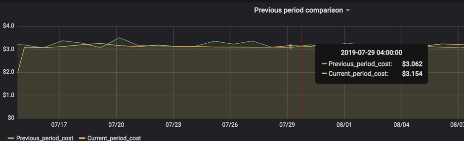
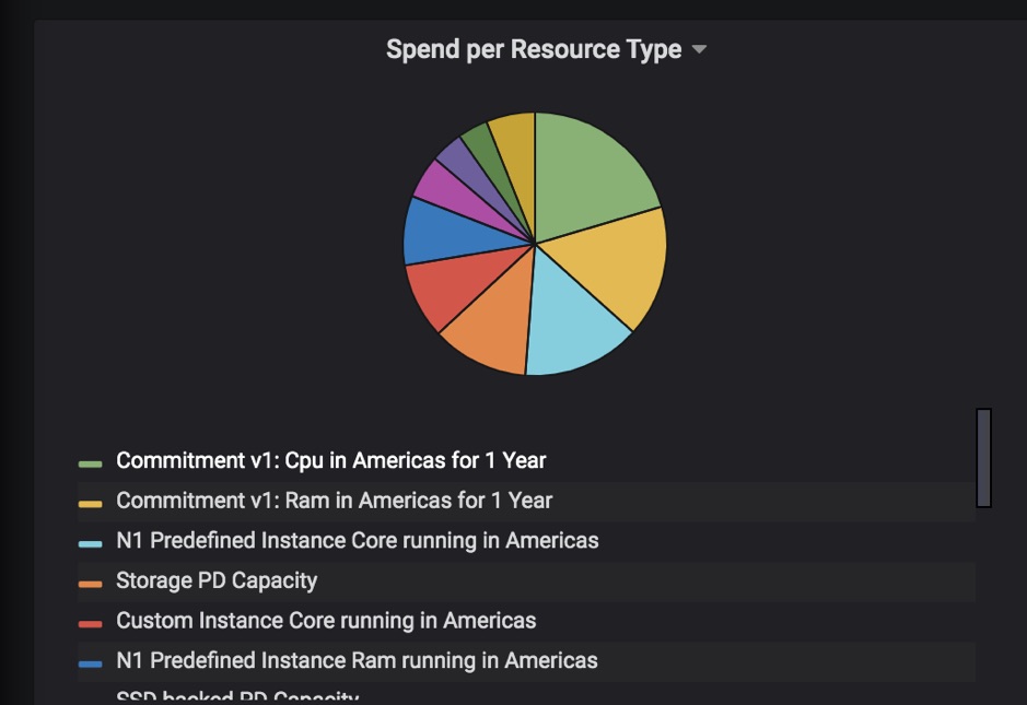
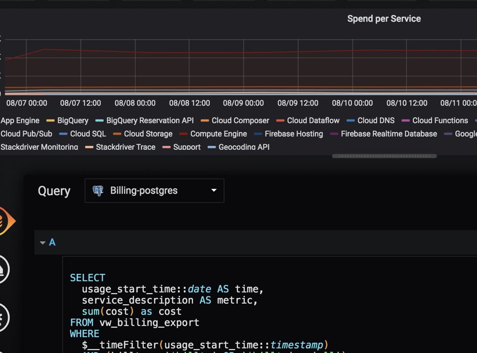
The last step was the creation of the Grafana dashboards. While we could use any charts that made sense, we used Data Studio Billing Report Demo as inspiration (of course we had to write all SQL queries from scratch).
Using a separate user in the database with read-only access to the view with billing data and to connect from Grafana is recommended as a security best practice.
Here are some examples of charts.
Summary
The above is a walkthrough of how we implemented a workflow to visualize billing data. The mechanism also supports adding new filters and metrics. At implementation roll-out, the client got a set of useful and fast dashboards that help to monitor Google Cloud spending. With this insight, the client is now empowered to make further cost optimizations.
Written by Dariia Vasilenko
How do manage your cloud spending? Are you wondering if you have workloads that can be optimized? Please let us know at [email protected]. We’d love to hear from you!